The basic idea of a Feature Extractor Feedback System (FEFS) is to have an audio signal generator whose output is analysed with some feature extractor, and this time varying feature is mapped to control parameters of the signal generator in a feedback loop.

What would be the simplest possible FEFS that still is capable of a wide range of sounds? Any FEFS must have the three components: a generator, a feature extractor and a mapping from signal descriptors to synthesis parameters. As for the simplicity of a model, one way to assess it would be to formulate it as a dynamic system and count its dimension, i.e. the number of state variables.
Although FEFS were originally explored as discrete time systems, some variants can be designed using ordinary differential equations. The generators are simply some type of oscillator, but it may be less straightforward to implement the feature extractor in terms of ordinary differential equations. However, the feature extractor (also called signal descriptor) does not have to be very complicated.
One of the simplest possible signal descriptors is an envelope follower that measures the sound's amplitude as it changes over time. An envelope follower can be easily constructed using differential equations. The idea is simply to appy a lowpass filter (as described in a previous post) to the squared input signal.
For the signal generator, let us consider a sinusoidal oscillator with variable amplitude and frequency. Although a single oscillator could be used for a FEFS, here we will consider a system of N circularly connected oscillators.
The amplitude follower introduces slow changes to the oscillator's control parameters. Since the amplitude follower changes smoothly, the synthesis parameters will follow the same slow, smooth rhythm. In this system, we will use a discontinuous mapping from the measured amplitudes of each oscillator to their amplitudes and frequencies. To this end, the mapping will be based on the relative measured amplitudes of pairs of adjacent oscillators (remember, the oscillators are positioned on a circle).
Let g(A) be the mapping function. The full system is
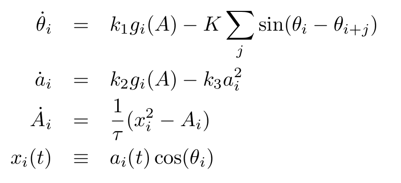
with control parameters k1, k2, k1, K and τ. The variables θ are the oscillators' phases, a are the amplitude control parameters, A is the output of the envelope follower, and x(t) is the output signal. Since x(t) is an N-dimensional vector, any mixture of the N signals can be used as output.
Let the mapping function be defined as

where U is Heaviside's step function and bj is a set of coefficients. Whenever the amplitude of an oscillator grows past the amplitude of its neighboring oscillators, the value of the functions g changes, but as long as the relative amplitudes stay within the same order relation, g remains constant. Thus, with a sufficiently slow amplitude envelope follower, g should remain constant for relatively long periods before switching to a new state. In the first equation which governs the oscillators' phases, the g functions determine the frequencies together with a coupling between oscillators. This coupling term is the same as is used in the Kuramoto model, but here it is usually restricted to two other oscillators. The amplitude a grows at a speed determined by g but is kept in check by the quadratic damping term.
Although this model has many parameters to tweak, some general observations can be made. The system is designed to facilitate a kind of instability, where the discontinuous function g may tip the system over in a new state even after it may appear to have settled on some steady state. Note that there is a finite number of possible values for the function g: since U(x) is either 0 or 1, the number of distinct states is at most 2N for N oscillators. (The system's dimension is 3N; the x variable in the last equation is really just a notational convenience.)
There may be periods of rapid alteration between two states of g. There may also be periodic patterns that cycle through more than two states. Over longer time spans the system is likely to go through a number of different patterns, including dwelling a long time in one state.
Let S be the total number of states visited by the system, given its parameter values and specific initial conditions. Then S/2N is the relative number of visited states. It can be conjectured that the relative number of states visited should decrease as the system's dimension increases. Or does it just take much longer time for the system to explore all of the available states as N grows?
The coupling term may induce synchronisation between the oscillators, but on the other hand it may also make the system's behaviour more complex. Without coupling, each oscillator would only be able to run at a discrete set of frequencies as determined by the mapping function. But with a non-zero couping, the instantaneous frequencies will be pushed up or down depending on the phases of the linked oscillators. The coupling term is an example of the seemingly trivial fact that adding structural complexity to the model increases its behavioural complexity.
There are many papers on coupled systems of oscillators such as the Kuramoto model, but typically the oscillators interact through their phase variables. In the above model, the interaction is mediated through a function of the waveform, as well as directly between the phases through the coupling term. Therefore the choice of waveform should influence the dynamics, which indeed has been found to be the case.
With all the free choices of parameters, of the b coefficients, the waveform and the coupling topology, this model allows for a large set of concrete instantiations. It is not the simplest conceivable example of a FEFS, but still its full description fits in a few equations and coefficients, while it is capable of seemingly unpredictable behaviour over very long time spans.
With all the free choices of parameters, of the b coefficients, the waveform and the coupling topology, this model allows for a large set of concrete instantiations. It is not the simplest conceivable example of a FEFS, but still its full description fits in a few equations and coefficients, while it is capable of seemingly unpredictable behaviour over very long time spans.
