Formulating a Feature Extractor Feedback System as an Ordinary Differential Equation

The basic idea of a Feature Extractor Feedback System (FEFS) is to have an audio signal generator whose output is analysed with some feature extractor, and this time varying feature is mapped to control parameters of the signal generator in a feedback loop.

What would be the simplest possible FEFS that still is capable of a wide range of sounds? Any FEFS must have the three components: a generator, a feature extractor and a mapping from signal descriptors to synthesis parameters. As for the simplicity of a model, one way to assess it would be to formulate it as a dynamic system and count its dimension, i.e. the number of state variables.

Although FEFS were originally explored as discrete time systems, some variants can be designed using ordinary differential equations. The generators are simply some type of oscillator, but it may be less straightforward to implement the feature extractor in terms of ordinary differential equations. However, the feature extractor (also called signal descriptor) does not have to be very complicated.

One of the simplest possible signal descriptors is an envelope follower that measures the sound's amplitude as it changes over time. An envelope follower can be easily constructed using differential equations. The idea is simply to appy a lowpass filter (as described in a previous post) to the squared input signal.

For the signal generator, let us consider a sinusoidal oscillator with variable amplitude and frequency. Although a single oscillator could be used for a FEFS, here we will consider a system of N circularly connected oscillators.

The amplitude follower introduces slow changes to the oscillator's control parameters. Since the amplitude follower changes smoothly, the synthesis parameters will follow the same slow, smooth rhythm. In this system, we will use a discontinuous mapping from the measured amplitudes of each oscillator to their amplitudes and frequencies. To this end, the mapping will be based on the relative measured amplitudes of pairs of adjacent oscillators (remember, the oscillators are positioned on a circle).

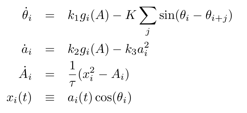
Let g(A) be the mapping function. The full system is

with control parameters k₁, k₂, k₁, K and τ. The variables θ are the oscillators' phases, a are the amplitude control parameters, A is the output of the envelope follower, and x(t) is the output signal. Since x(t) is an N-dimensional vector, any mixture of the N signals can be used as output.

Let the mapping function be defined as

where U is Heaviside's step function and b_j is a set of coefficients. Whenever the amplitude of an oscillator grows past the amplitude of its neighboring oscillators, the value of the functions g changes, but as long as the relative amplitudes stay within the same order relation, g remains constant. Thus, with a sufficiently slow amplitude envelope follower, g should remain constant for relatively long periods before switching to a new state. In the first equation which governs the oscillators' phases, the g functions determine the frequencies together with a coupling between oscillators. This coupling term is the same as is used in the Kuramoto model, but here it is usually restricted to two other oscillators. The amplitude a grows at a speed determined by g but is kept in check by the quadratic damping term.

Although this model has many parameters to tweak, some general observations can be made. The system is designed to facilitate a kind of instability, where the discontinuous function g may tip the system over in a new state even after it may appear to have settled on some steady state. Note that there is a finite number of possible values for the function g: since U(x) is either 0 or 1, the number of distinct states is at most 2^N for N oscillators. (The system's dimension is 3N; the x variable in the last equation is really just a notational convenience.)

There may be periods of rapid alteration between two states of g. There may also be periodic patterns that cycle through more than two states. Over longer time spans the system is likely to go through a number of different patterns, including dwelling a long time in one state.

Let S be the total number of states visited by the system, given its parameter values and specific initial conditions. Then S/2^N is the relative number of visited states. It can be conjectured that the relative number of states visited should decrease as the system's dimension increases. Or does it just take much longer time for the system to explore all of the available states as N grows?

The coupling term may induce synchronisation between the oscillators, but on the other hand it may also make the system's behaviour more complex. Without coupling, each oscillator would only be able to run at a discrete set of frequencies as determined by the mapping function. But with a non-zero couping, the instantaneous frequencies will be pushed up or down depending on the phases of the linked oscillators. The coupling term is an example of the seemingly trivial fact that adding structural complexity to the model increases its behavioural complexity.

There are many papers on coupled systems of oscillators such as the Kuramoto model, but typically the oscillators interact through their phase variables. In the above model, the interaction is mediated through a function of the waveform, as well as directly between the phases through the coupling term. Therefore the choice of waveform should influence the dynamics, which indeed has been found to be the case.

With all the free choices of parameters, of the b coefficients, the waveform and the coupling topology, this model allows for a large set of concrete instantiations. It is not the simplest conceivable example of a FEFS, but still its full description fits in a few equations and coefficients, while it is capable of seemingly unpredictable behaviour over very long time spans.

The theoretical minimum of physics

The theoretical minimum.

What you need to know to start doing physics

by Susskind and Hrabovsky, 2013

This crash course of classical mechanics is targeted at those who “regretted not taking physics at university” or who perhaps did but have forgotten most of it, or anyone who is just curious and wants to learn how to think like a physicist. Since first year university physics courses usually have rather high drop out frequencies, there must be some genuine difficulties to come over. Instead of dwelling on the mind-boggling paradoxes of quantum mechanics and relativity as most popular physics books do, and wrapping it up in fluffy metaphores and allusions to eastern philosophy, the theoretical minimum offers a glimpse of the actual calculations and their theoretical underpinnings in classical mechanics.

This two hundred page book grew out of a series of lectures given by Susskind, but adds a series of mathematical interludes that serve as refreshers on calculus. Although covering almost exactly the same material as the book, the lectures are a good complement. Some explanations may be more clear in the classroom, often prompted by questions from the audience. Although Susskind is accompanied by Hrabovsky as a second author, the text mysteriously addresses the reader in the first person singular.

A typical first semester physics text book may cover less theory than the theoretical minimum in a thousand pages volume, although it would probably cover relativity theory which is not discussed in this book. There are a few well chosen exercises in the theoretical minimum, some quite easy and a few that take some time to solve. “You can be dumb as hell and still solve the problem”, as Susskind puts it in one of the lectures while discussing the Lagrangian formulation of mechanics versus Newton's equations. That quote fits as a description of the exercises too, as many of them can be solved without really gaining a solid understanding of how it all works.

The book begins by introducing the concept of conservation of information and how it applies to deterministic, nonreversible systems (all systems considered in classical mechanics are deterministic and nonreversible). Halfways through the book the first more advanced ideas come into play: the Lagrangian and the principle of least action. In general, one gets an idea of what kinds of questions physicists care about, such as symmetries and conservation laws. Examples of symmetries that are discussed include spatial translation invariance and time shift invariance, and the conservation of energy is a recurrent theme. The trick is simple: take a time derivative of the Lagrangian or the Hamiltonian, and show it to be zero. The principle of least action requires more sophisticated mathematics (functional analysis), although the authors try to explain it in very simple terms. Nonetheless, that part is not very easy to follow.

The writing is concise, yet almost colloquial, with only a few typos. Mathematical rigour is thrown out whenever it would clutter the exposition. Susskind does not care for limits in the formulation of derivaties, but uses a delta or an epsilon that is supposedly infinitesimal in a loosely nonstandard analysis kind of way. Most derivations are easy to follow, using elementary calculus and patiently laid out step by step. Some background in one variable and vector calculus will be necessary to follow the text, although all math that is needed (which is not very much) is summarized in the mathematical interludes.

Why should we need to know about Lagrangians, Hamiltonians and Poisson brackets, a student may ask. Susskind's answer might be that Lagrangians make the solution of certain problems much easier than trying to apply Newton's equations, and that Hamiltonians play an important role in quantum mechanics.

The theoretical minimum is probably the most concise introduction to advanced physics out there, highly suitable for self-study. It provides much of the essential background needed for books reviewed here in previous posts, such as Steeb's Nonlinear Workbook or Haken's Synergetics.

How to patch your own oscillator

The charming world of analog modular synthesis offers many choices regarding how to construct one's instrument from components. There are lots of oscillators, filters, VCAs, LFOs, signal processors and utility modules to choose among. In that setting, it can be very interesting to build something as elementary as an oscillator out of even more basic components. Here is an example of how it can be done with two modules, neither of which functions as an oscillator on its own.

The modules needed are a utility module that mixes, offsets and inverts signals, and a dual slew limiter (or two separate slew limiters). In particular, this example will work with Doepfer's Slew Limiter A-170 SL and wmd's Invert Offset mk II. However, there is nothing magic about these modules, so other modules that offer equivalent functionality may replace them.

Five patch cords are needed to connect the modules as illustrated. Then, with some tweaking of the knobs, slow oscillations should occur. It is possible to influence the frequency by the settings of all the knobs. By adjusting the two lower knobs of A-170, controlling the rise and fall times, the wave shape can also be varied from rising ramp through triangle to falling ramp. The amplitude may be low, and the frequency usually sub-audio, although low bass frequencies in the audio range can be obtained. The effects are best observed if the CV out of the Invert Offset is routed to the frequency input of another oscillator.

What is actually going on in this patch? To a first approximation, the slew limiter can be regarded as an integrator. In fact, it is probably more accurate to think of it as a leaky integrator. The Invert Offset consists of two identical blocks with two signal inputs and two outputs each. Let us introduce the labels x₊, x_-, y₊ and y_- for the output signals, and u_x, u_y, v_x and v_y for the inputs, as shown in the sketch above. The knobs, labeled c_x and c_y, add a constant offset to the signal. Inferring from the user's manual, the following set of equations should describe what the module does.

Expressing the action of the slew limiter as an integral, and following the patch cords that go into the inputs of the Invert Offset module, the system is given by:

After a number of substitutions, and taking derivatives to get rid of the integrals, the system simplifies to:

If the constants are both zero, the eigenvalues of this system are 1±i, indicating that the system is unstable. Clearly something in the model is wrong, since the actual patch does not blow up in any way. As hinted at earlier, the slew limiters do not actually integrate the signal. If they did, there would be infinite gain at dc so any constant signal fed into one of them would keep increasing linearly. What happens in reality is that, starting from a relaxed state and feeding a constant signal into a slew limiter, the output grows from zero until it reaches the level of the input. If one had two true integrators and an inverter, the equations for an harmonic oscillator

could be realized quite easily. 

The moral of this failed attempt at modeling two quite simple modules is that even seemingly simple modules may hide more complex behaviour than one would naively suspect. In any case, it may be surprising to find that five patch cords connecting these modules in the right way are all it takes to turn them into a low frequency oscillator. Although there are more than one way to patch up an oscillator from these two modules, there are many more ways to patch up systems that do not oscillate. Bistable systems with hysteresis is the result in most cases.

Synergetics, the book

Hermann Haken: Synergetics. Introduction and Advanced Topics. 

[Disclaimer: There are many things in this book that I do not understand, although hopefully I have grasped the big picture.]

Under the term Synergetics, Haken collects a number of approaches that can be useful in a variety of scientific disciplines ranging from physics, chemistry and biology, to economics and even sociology. Synergetics is presented as its own discipline with its characteristic concepts and methods. Yet this discipline draws on related fields such as thermodynamics, statistical dynamics, information theory, dynamic systems, control theory, bifurcations and catastrophe theory. Synergetics proposes to shed light on self-organized phenomena in various areas and to treat them within a unified apparatus. In particular, the slaving principle is the one trick that is used again and again. The slaving principle can be thought of in terms of a dynamic system where some variables change fast and others slowly, but there is also a separation into stable and unstable modes. The stable modes can be eliminated and treated as parameters, resulting in great simplifications.

This tome contains two classic volumes in one. Volume one (Introduction) begins gently with tutorial chapters on basic probability theory, ordinary differential equations, and their combination in stochastic differential equations. After the theoretical background has been presented, there is a chapter on self-organization followed by several chapters devoted to applications in various domains. First, the chapter on physics deals mainly with lasers. Then, as the chapters turn to chemistry, biology and economics in turn, the treatment becomes more and more accessible to the non-specialist. However, at the same time the models seem to become increasingly simplistic. Already the examples from biology and population dynamics are sketchy, and the discussion of applications to economics and sociology do not introduce many useful ideas. Nonetheless, one should remember that Haken was among the pioneers who brought a physicist's tool kit to these fields. In particular,

[...] synergetics has established links between dynamic systems theory and statistical physics. Undoubtedly, the marriage between these two disciplines has started. (p. 364 of the double volume) 

Further, regarding the connections of physics, chemistry, biology and even softer sciences:

It thus appears that we are presently from two different sides digging a tunnel under a big mountain which has so far separated different disciplines, in particular the “soft” from the “hard” sciences. (p. 364-5) 

We see the results of this excavation in numerous papers today, where physicists have begun to address such problems as the motion of crowds at concerts or the opinion formation before elections. However, there are obvious dangers involved in attacking problems that lie far beyond one's sphere of specialization. In the words of Buckminster Fuller (who also wrote a two volume book called Synergetics, otherwise bearing little resemblance to Haken's):

The word generalization in literature usually means covering too much territory too thinly to be persuasive, let alone convincing. In science, however, a generalization means a principle that has been found to hold true in every special case.

Apparently both kinds of generalization are involved in Hakens work; the applicability seems to decrease the further away from physics one gets, till it begins to look suspicious when applied to the social sciences. Meanwhile, the single finding that unites all chapters, the slaving principle, exemplifies the kind of generalization that holds true in several special cases, if not in all conceivable scenarios. It is the method of finding solutions that survives generalizations, not necessarily so with the modelling of systems in different fields.

Volume two (Advanced Topics) starts over with a long expository chapter on the application domains followed by the introduction of the theory. There are short sections on deterministic chaos, but Haken is not the best source on this. Quasi-periodicity is treated extensively. Although the exposition is clear to begin with, soon enough matters get complicated. If you ever wondered what makes a system of differential equations with quasi-periodic coefficients stable or unstable, this is the text to read.

Matters of style

The first chapters of each volume are tutorial in character and cover material that most readers probably already know. The manner of exposition changes as Haken begins to introduce his own findings—one can sense a shifting of gears when his enthusiasm sets in. Unfortunately, these parts involve solutions that stretch over sections or entire chapters, sometimes using idiosyncratic notation. It is often hard to tell whether a variable is supposed to be real, complex, or a vector, even though one may be able to figure it out from the context.

The writing has the appearance of a stream of consciousness layed out at the blackboard, rather than elaborated at the typing machine. Throughout the book, variable substitutions are profusely employed; so much, in fact, that one almost inevitably loses track of the variables' meaning. The derivations are decidedly informal, with almost no theorems and proofs. (There are a handful of theorems that rely on a long list of assumptions with long, unwieldy proofs.) Instead there are long chains of “simplifications” or “abbreviations”, often resulting in expressions that are longer than the one they replace, truncations of higher order terms in series expansions and other sorts of approximations. All these tricks are of course what physicists are usually good at, but for readers without the proper background, they may appear as incomprehensible as pulling rabbits out of a hat.

If synergetics has to do with self-organization of complex systems, it must be said that Haken is quite terse on the topic of self-organization as such. This is where some conceptual analysis is lacking. On the other hand, the cyberneticians have already contributed much hand-waving philosophizing on self-organization, without necessarily having contributed much to its understanding. Here, at least, one has a class of problems and an approach to their solution, but there is more to self-organization than what is covered in this book.

Oscilloscopes, phase plots and beyond

Similarly to how oscilloscopes trace out two signals x(t) and y(t), one might plot any related variables against each other.

The above illustration shows x(t) against y(t), both of which seem to be periodic, albeit quite complicated waveforms.

Phase plots of, say, position versus momentum are another common way to display orbits of differential equations. Any recorded signal may be plotted with its numerically estimated derivative on the y-axis. Hint: use a higher order differentiating filter, not just a forward or backward difference.

Graphs of the amplitude spectrum of one signal against that of another signal are harder to interpret. The axes then represent amplitudes, and each point is a unique frequency whose coordinates is the amplitude in signal x versus its amplitude in signal y. If the points gather near a thin line along the main diagonal, the two spectra are highly correlated.

Another novel kind of plot is the signed amplitude spectrum. It combines phase information with the amplitude spectrum and distinguishes positive and negative amplitues depending on the sign of the phase. Below, the red line is the signed amplitude spectrum of one variable and the blue line is that of a related variable in the same system.

All the illustrations come from a 3D ODE that is currently under investigation, suspected guilty of exhibiting interesting behaviour.

Filtering with differential equations

For those of us who are more familiar with digital filters than their analog counterparts, a one pole lowpass filter is easy:

y_n = (1 - β)x_n + βy_n-1,   0 < β < 1.

But how do you filter a signal with an ordinary differential equation?



Working backwards, we should have an ODE that says

dy/dt + Ay(t) = Bx(t)   (*)

for some suitable constants A and B yet to be found. The differential may be approximated with a forward difference over a short time interval T, so dy(nT)/dt ≈ (y(nT+T) - y(nT))/T. Setting T equal to one sampling period, the discrete time version of (*) is

(y_n+1 - y_n)/T + ay_n = bx_n. 

Perform some algebraic shuffling to and fro of the variables to obtain

y_n+1 = bTx_n + (1 - aT)y_n

and recall that the filter coefficients are 1 - β = bT and β = 1 - aT, hence bT = aT. Now we introduce a new coefficient τ > 0 for the variables in (*) and set 1/τ equal to both A and B. The system then is

dy/dt = (x - y) / τ

where now τ plays the role of a relaxation time constant. The greater τ is, the slower the response of the filter. Also, when the input equals the output the derivative becomes zero, which is to say that the system has unit DC response as required.